Master recipe: How to learn your machines
These are notes I made while I was taking the Deeplearning.ai Deep Learning Specialization, more specifically, the awesome Improving Deep Neural Networks: Hyperparameter tuning, Regularization and Optimization course, through which Andrew Ng lays down a basic recipe for training your machines! I highly recommend you taking it, it's free and you'll absolutely learn something even if you're an experienced ML practicioner.
This may very well be the most useful part of my project. Be sure to at least take a look. 🙂
Preparing your data
One of the first questions while preparing you should answer is how to split your dataset? One good practice is to split the data into three parts;
Training set, cross validation/dev set and test set.
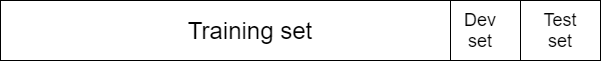
- You train the data on the training set, and validate it using the dev set.
- Since you're using the dev set to tune the model hyperparameters, you're kinda fitting them to the data in the dev set. That's why after you've chosen the exact hyperparameters you want and after you've completely trained your model, you should test it using the test set, which is data it has never ever seen before, and should give you a “real-world” benchmark on how it performs.
How to split the data (size-wise):
- If you have a small amount of data, in the tens of thousands, you can use the “olden” way (pre big-data) of splitting the data: 60% for your training set, 20% for your dev and 20% for your test set
- If however your data is in the millions, using 20% or 200 000 examples for your dev and test is surely a bit of an overkill. You can decide to use something like 10 000 examples for your dev/test sets, so you'd have a split of 99%/1%/1% for your train/dev/test sets respectively.
- If your dataset is even bigger, you can also use something like 99.5%/0.4%/0.1%, whatever lets you quickly decide how well the model is training and performing on data it's never seen before.
Make sure your training and dev/test sets come from the same distribution.
-
If your training data is really high res, but the data you'll use during inference is lower quality due to lower resolutions, shaky camera, dirty lenses, and so on, your model won't perform well.
-
Your training data should be as similar as possible to real world data you'll use during inference, and you should try to cover as much possible situations you can, which includes different weather conditions, bumpy roads, and so on.
-
The main reason for this type of mismatch is that you don't have enough training data, so you get some online, e.g. if you took a YouTube video of a car driving around town that has a super high res camera and added it to your training data, but your RC car has a really low res camera.
How to know if your model has high variance or bias (or both):
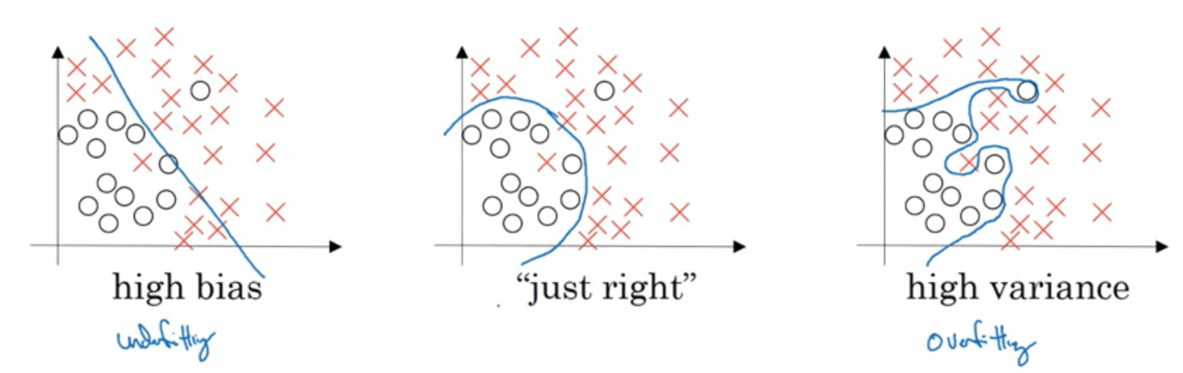
Here's a great illustration by Andrew Ng on what high bias and variance look like:
-
High variance: the model is overfitting the training data and performing poorly on new unseen data.
-
High bias: the model isn't even performing well on the training data.
-
High bias and high variance: the model underfits the training data but performs even worse on the dev data.
The two key things to take away are:
-
By looking at how well the model performs on the training data, you can see how much bias it has; if it has a low error, it has a low bias, if it has a large error, it has large bias.
-
By looking at how well the model performs on the dev set, you can see how much variance it has; if it performs much worse than on the training set, it has high variance, if it performs slightly worse or the same, it has low variance and generalizes well.
Basic recipe for learning your machines
- Get the model to perform well on the training data (low bias)
- Get the model to perform well on the dev set data (low variance)
If you have large bias:
- (Almost always works): Try a bigger network: more hidden layers, more hidden units.
- (Sometimes works, but never hurts): Try training it longer: give it more time or use more advanced optimization algorithms.
- (Maybe it'll work, maybe it won't): Try finding a better neural net architecture: try finding an architecture that's proven to work for your specific problem.
- Consider asking yourself: is this even possible to do? If you're trying to train a classifier on very blurry low res images, is it even possible to do so? What's the base error for that problem?
If you have large variance:
- (Best way to solve it): Get more data, it can only help. But sometimes it's impossible to get more data.
- (Almost always helps): Regularization
- (Maybe it'll work, maybe it won't): Try finding a better neural net architecture. Same as for the large bias problem.
Don't worry about the bias-variance tradeoff if you're doing deep learning. It isn't much of a thing anymore:
- As long as you can train a bigger network (and use regularization), you'll almost certainly be able to get rid of high bias without increasing variance (by much).
- As long as you can get more data (not always, but mostly possible), you'll almost certainly be able to get rid of high variance without increasing bias (by much).
Regularizing neural nets
To try and gain some intuition about regularization in neural nets, let's walk through implementing L2 regularization in a neural net. Since we're mostly doing computer vision stuff with our self-driving car, we'll most likely be using batch normalization and dropout regularization rather than L2, which is used much more often in computer vision, so feel free to skip this part if you're not interested.
If our cost function is defined as:
The first part uses the regularization parameter $\lambda$, which is a hyperparameter to be tuned using the dev set, and divides it by $2n$, which is just a scaling constant.
The second part uses the Frobenius norm (basically the L2 norm of a matrix), and it basically sums up the squares of all the elements of all $\mathcal{w}$ matrices we use:
When implemented, during backprop the $W^{[l]}$ matrix gets multiplied by $\frac{\lambda}{n}$, a number slightly smaller than 1, which is why it's also called weight decay, since the weight loses just a bit of it's value.
Why does this help?
If we set the $\lambda$ parameter in the regularization term below to a large value, it will set the values of $w^{[l]}$ very close to zero.
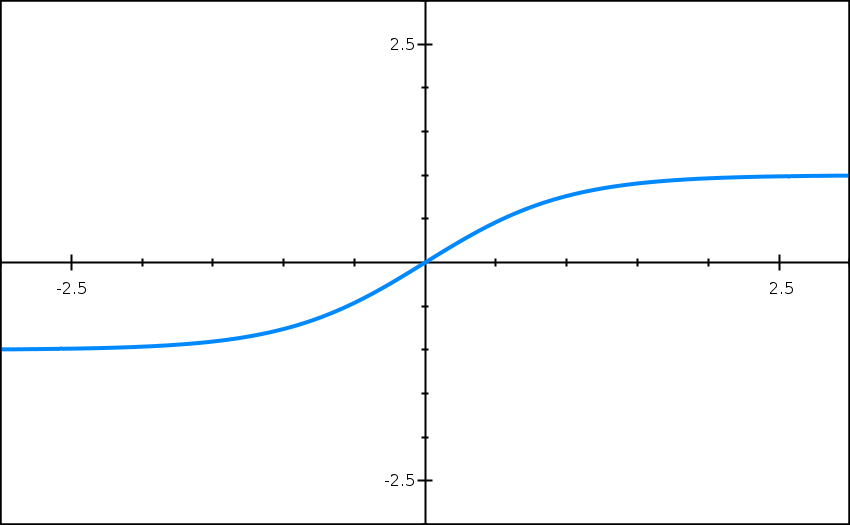
If the value of $z^{[l]}$ can be only a small range of values close to zero, our activation function will start looking like a linear function, as shown below:
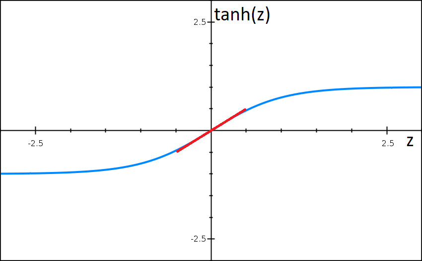
Which in turn means every layer in our neural net will begin to look like a linear layer, which will cause our network to be able to approximate only a linear function to our data, which will cause our model to go from high variance to high bias.
Of course, we don't (and won't) set our $\lambda$ parameter to a very large value, but rather set it to somewhere in between, which will get rid of our high variance problem and not cause high bias instead.
Dropout regularization
This illustration was also taken from Andrew Ng's course video:
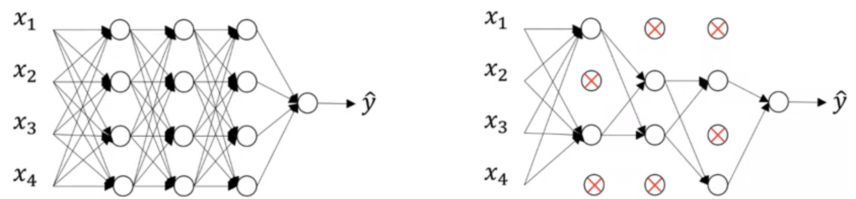
Imagine we have a neural net that looks like the one pictured above, on the left.
To stop our model from overfitting our data, we can randomly knock-out some neurons while training our model. This in turn causes the model to be unable to rely on just a particular set of neurons, or a pathway of neurons, so it has to train multiple subsets of neural nets, which makes it much more difficult to overfit the data, since it never knows when some of the neurons will be knocked out. $$ S(i,j) = (I*K)(i,j) = \sum_m\sum_nI(m,n)K(i-m,j-n) $$
Other tips to prevent overfitting/bias
Augment your data
Let's say we're training our car on the following track:
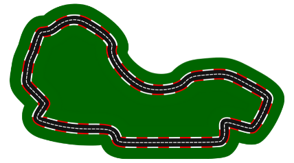
We run a few laps on the track and save our data. If we've only driven in the usual, counter-clockwise direction, we have inadvertently caused our model to be slightly biased to always turn a bit to the left.
Why?
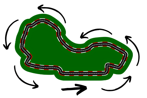
We can see that, globally, the car is always turning a bit to the left. So if you only include this data in your training set, the car will always be inclined to turn just a bit to the left.
How to solve it
Other than driving the very same track, just in the opposite direction, you can simply mitigate this issue by augmenting your data with the same images, just horizontally flipped, thus getting:
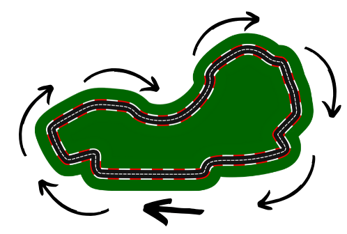
Now your car shouldn't be inclined much to steer to one side or the other for no reason.
Make sure to make copies of your JSON files and invert their steering values as well.
Augmentation by Neural Style transfer
You can even apply preprocessing like this to your images to try and make it focus on the more important features such as lane lines:


Also, I wrote this just to have an excuse to make some artful Baby Yoda memes, which had to be put into this project somehow, so here goes:


You could still tell that it's Baby Yoda, even though the images lost a lot of the original information about him, e.g. the hairs on his head. So in contrast, you could use this approach and still be able to identify lane lines on images, but just by focusing on the things that make us recognize them the most.
Or not. Anyways, artful Baby Yoda memes.
Early stopping
When training your model, you can often see the validation error getting lower over time, following the training error curve, but then at one moment you see it take off and get much worse over time:
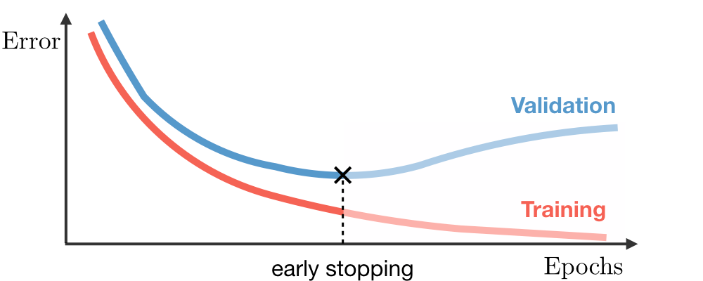
One possible solution is stopping the training early, when you see the validation error starting to increase.
Just keep in mind that by doing so, you're now coupling two optimization problems that you were solving as separate before: the optimization of your cost function and the prevention of overfitting the dataset. By doing so, you're not doing quite the best job you could at minimizing the cost function, since it's obvious that the error could get much lower if the training wasn't stopped early, while you're simultaneously trying not to overfit your data.
One alternative could be using L2 regularization or some other regularization technique, but you can often see early stopping being used in practice. Just keep in mind the trade off you're doing.
Iterating quicker: a single number performance metric
First, lets define two terms using a classifier example; precision and recall.
Precision: of the examples that your classifier recognizes as X, how many examples actually are X. Recall: of the examples that are actually X, how many of them does your classifier recognize as X.
We can combine these two metrics into a single number, as a harmonic mean of the two, which is called the F1 score:
But imagine trying to decide between three implementations of a classifier with 3 possible classes:
| Implementation/Classes | A (precision) | A (recall) | B (precision) | B (recall) | C (precision) | C (recall) |
|---|---|---|---|---|---|---|
| First implementation | 95% | 90% | 89% | 88% | 92% | 89% |
| Second implementation | 93% | 89% | 92% | 90% | 92% | 90% |
| Third implementation | 89% | 88% | 95% | 93% | 90% | 89% |
Which one is the best? Sure isn't easy to tell from the table above. At least not to me.
Now look what it would look like if we used the F1 score for all of the possible classes:
| Implementation/Classes | A ($F_1$ score) | B ($F_1$ score) | C ($F_1$ score) |
|---|---|---|---|
| First implementation | 92.4% | 88.5% | 90.5% |
| Second implementation | 91% | 91% | 91% |
| Third implementation | 88.5% | 94% | 89.5% |
Looks much simpler than the first table, but still could be simpler. Since we're probably interested in our classifier working as best as possible over all classes, we can take the average of all of the 3 $F_1$ scores to get one simple number that tells us how well our classifier works:
| Implementation/Classes | Average $F_1$ score |
|---|---|
| First implementation | 90.5% |
| Second implementation | 91% |
| Third implementation | 90.7% |
Why do this?
The example above could've easily had a hundred different classes, with a dozen different implementations. That would've been impossible to look at even if you used $F_1$ scores for every class.
When trying out a bunch of different values of hyperparameters and implementation details, it's much faster to iterate and much easier to decide between all possible implementations when you have a single number that tells you how well it performs. And I believe this is a pretty good way to get one, even considering the amount of some fine-grained details you lose. You can always look them up after you eliminate some implementations, and have only a few you're actually considering.
One important thing to notice is that there could be other important metrics to look at other than how accurate our classifier is.
For an example, we could be making a classifier that classifies obstacles our car will collide with if we don't avoid them. Surely, we'd like to correctly classify as much of those as possible, so make a table, as the one above:
| Classifier/Score | $F_1$ score |
|---|---|
| First classifier | 92% |
| Second classifier | 97% |
| Third classifier | 99% |
Cool, so we pick the third classifier. And our car crashes. Wait, wut?
We picked the best classifier in terms of it correctly classifying as much of the objects in our path as possible, but there's one thing we didn't look at; the time it takes it to classify an object.
| Classifier/Score | $F_1$ score | Average runtime |
|---|---|---|
| First classifier | 92% | 20 ms |
| Second classifier | 97% | 70 ms |
| Third classifier | 99% | 3000 ms |
So yeah, we did recognize most of the objects we were on a collision path with, but by the time that we did, the car had already crashed into them.
Taking that in mind, the second classifier is obviously the better choice.
So it's important to keep in mind that while we're trying to optimize one of the metrics of our model, we also have to pay attention to the other minimum requirements the model must have in order to actually be usable in the real world, as per our real-time necessary example.
Choosing Hyperparameters
Hyperparameters ordered by importance are:
- learning rate (alpha)
- beta, number of hidden units, mini-batch size
- number of layers, learning rate decay
A traditional way to choose hyperparameters is to sample them from a grid:
First we'd define a grid, which can either be a randomized or a regular grid, and then iteratively sample the parameters from it:
Illustration by Andrew Ng:
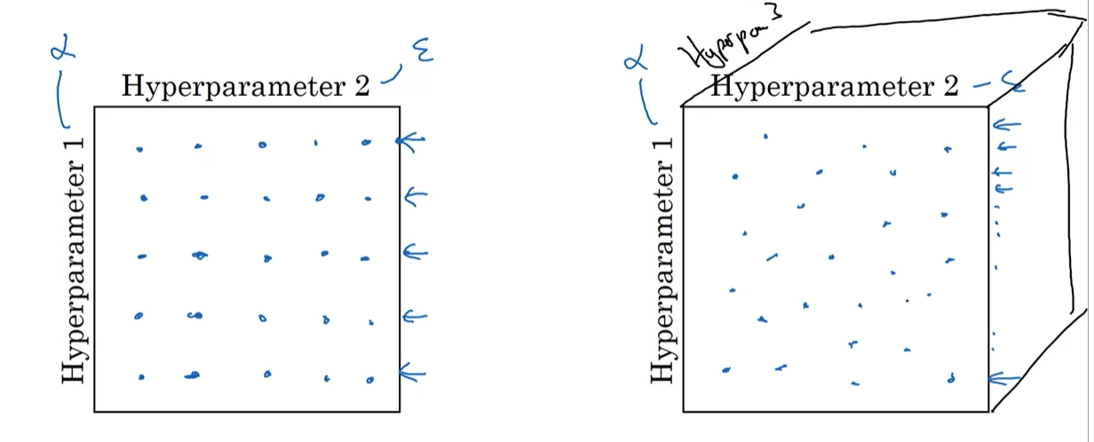
Keep in mind that the grid search approach suffers from the curse of dimensionality.
There's a lot of ways to do this, most frameworks even have built-in ways of doing this so I'd highly recommend you look into the topic of hyperparameter optimization.
Hyperparameters can get stale
Also keep in mind that you should re-evaluate your hyperparameters every once in a while, because as you get a lot more data, they can get stale.
They can also get stale if you get a new GPU/CPU, change your network a bit or for any number of reasons. Just re-evaluate them from time to time, depending on how much you're changing stuff around.
Closing thoughts
The more you do this stuff, the easier it'll get, and the more tricks you'll learn.
The thing about ML is that you have to rely on your intuition a lot. If a model is misbehaving, you can't simply set a breakpoint on it and debug it, there can be a plethora of reasons for it:
- Maybe your data is bad
- Maybe there is a bug in your architecture
- Maybe you're just using the wrong hyperparameters
- …
You have to keep trying and not give up. It can take a few days even to get your model to perform well, even on smaller testing datasets, depending on the complexity of the task you're trying to achieve.
Do your best to make sure that the things that you can control, e.g. the quality of your data and its distribution, are okay.
For the parts you can't directly see, like how your convolutional layers are doing stuff, you can use all sorts of tools like the visualization techniques we've done earlier to try and gain some intuition on how it's performing and what could go wrong.
That's pretty much it! Have fun experimenting with your model.
Next up: learning behaviours, e.g. lane changing!