Finding lane lines easier
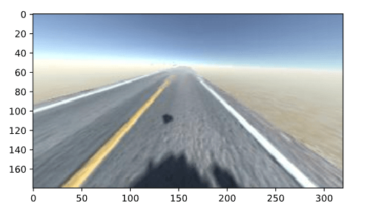
Remember we've showed before that our CNN is taking the horizon as the input feature, and that we'll be addressing it after making a simulator mod that'll allow us to take high res images. Well, here we are.
What we're going to do
To solve the horizon problem and simultaneously help the car recognize lane lines better, we'll do the following:
- Perform a perspective transform on every input image to get a birds-eye view of the road
- Convert the image to HLS color space, extract only the S channel and perform some thresholding on it to extract only the lanes from the input image
Perspective transform
There's one really useful thing we can do with our input images, and we kinda already did it while we were calibrating our camera; a perspective transform. So, what's a perspective transform? Let's say that this is our input image:
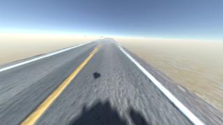
We talked a bit about how cameras map the 3D world onto a 2D plane, which certainly has some downsides. One of them would be this:
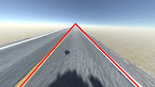
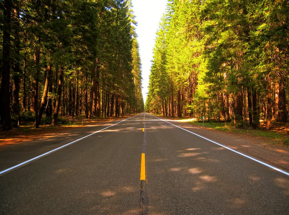
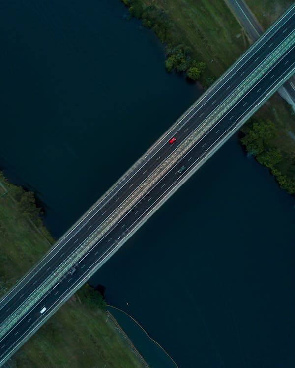
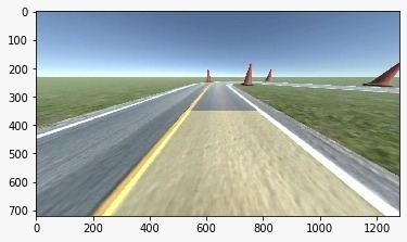
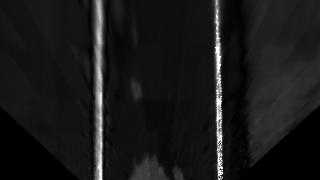
We know that the lane lines in the real world are parallel, but if the only input information we had was the image above, we could easily assume that they intersect somewhere in the distance. Maybe it's easier to see on a photo of a real road:
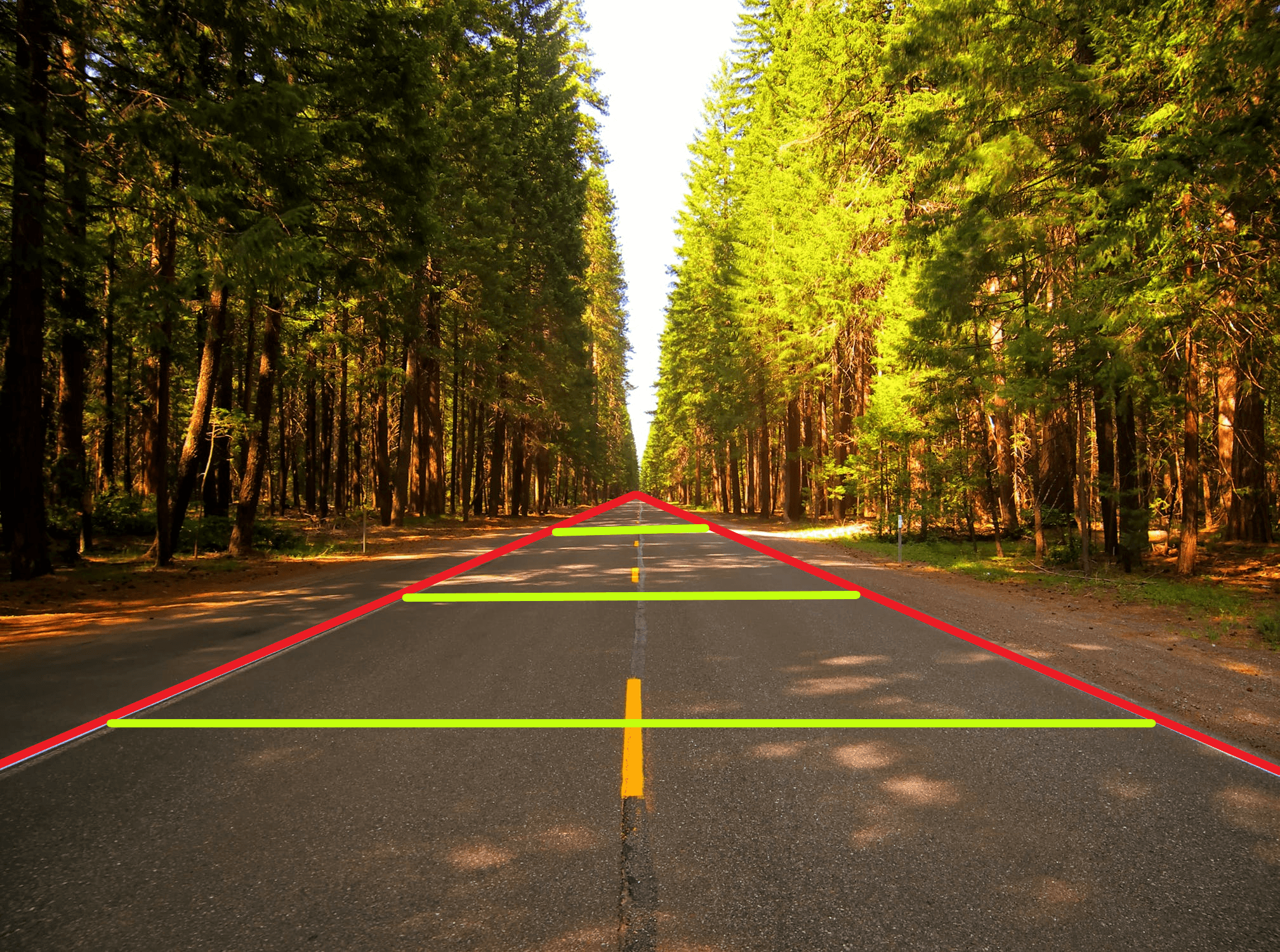
We could easily assume that the road gets narrower and narrower further on, until the outer lines intersect somewhere in the distance.
Now, if we had a birds-eye perspective, like this:
We could easily see that the lane lines are parallel throughout the road, and that the width of a lane should stay the same.
Luckily for us, we don't have to train an autonomous drone to fly above our car and send images of the road to it, we can just do a perspective transform, and go from this:

To this:
Implementing the perspective transform
As always, we'll be importing the stuff we need first, we'll be using numpy and OpenCV (and matplotlib for plotting the images in our Jupyter notebook, which you can download at the bottom of this page):
import numpy as np
import cv2
import matplotlib.pyplot as plt
%matplotlib inline
Since we're working in an Jupyter notebook and we're mixing OpenCV with matplotlib, we'll define some helper functions for showing our images, to make our code shorter and cleaner:
# So we don't have to use cv2.cvtColor everytime
def showImage(image):
    plt.figure()
    plt.imshow(cv2.cvtColor(image, cv2.COLOR_BGR2RGB))

# So we can show titled images too
def showTitledImage(title, image):
    plt.figure()
    plt.imshow(cv2.cvtColor(image, cv2.COLOR_BGR2RGB))
    plt.title(title)
    plt.axis('off')
Now we can open our image:
image = cv2.imread('path/toYour/image.jpg')
showImage(image)
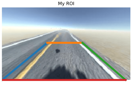
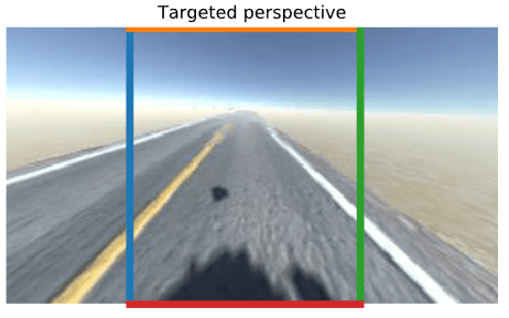
Next, we'll need to define the region of interest on our input image that we'd like to transform into our birds-eye perspective. You can get these coordinates by opening your image in an image editor and manually selecting the pixels that denote four edges of your ROI.
To help you better understand, here's an image of my ROI:
Next, you should write down the pixel coordinates of each corner of your image into an numpy array:
# Define the region of the image we're interested in transforming
regionOfInterest = np.float32(
                [[0,  180],  # Bottom left
                [112.5, 87.5], # Top left
                [200, 87.5], # Top right
                [307.5, 180]]) # Bottom right
To clarify, my bottom left coordinate is the pixel where the red and the blue line intersect, whose position is (0, 180). The same goes for the three remaining corners.
I'd like that the selected ROI looks like a square after the transform, where the left and right lane lines are parallel to each other, so I've defined my target perspective coordinates to look like:
The numpy array containing those coordinates looks like:
# Define the destination coordinates for the perspective transform
newPerspective = np.float32(
            [[80,  180],  # Bottom left
            [80,    0.25],  # Top left
            [230,   0.25],  # Top right
            [230, 180]]) # Bottom right
So both arrays look like:
# Define the region of the image we're interested in transforming
regionOfInterest = np.float32(
                [[0,  180],  # Bottom left
                [112.5, 87.5], # Top left
                [200, 87.5], # Top right
                [307.5, 180]]) # Bottom right

# Define the destination coordinates for the perspective transform
newPerspective = np.float32(
            [[80,  180],  # Bottom left
            [80,    0.25],  # Top left
            [230,   0.25],  # Top right
            [230, 180]]) # Bottom right
If you'd like to visualize your coordinate arrays by drawing lines over the original image like I did above, you can use the following function:
# Function that draws coordinates on an image, connecting them by lines
def drawLinesFromCoordinates(coordinates):
    # Pair first point with second, second with third, etc.
    points = zip(coordinates, np.roll(coordinates, -1, axis=0))
    # Connect point1 with point2: plt.plot([x1, x2], [y1, y2])
    for point1, point2 in points:
        plt.plot([point1[0], point2[0]], [point1[1], point2[1]], linewidth=5)
And call it like:
# Draw the image to visualize the selected region of interest
showTitledImage("My ROI", image)
drawLinesFromCoordinates(regionOfInterest)
Once you have your coordinates set, that's actually it. The rest of the implementation just calls a couple OpenCV functions, the first of which is cv2.getPerspectiveTransform, which takes in the starting coordinates we've defined (our ROI) and the target coordinates and gives us back a matrix with which we can warp our image to the target perspective.
This actually isn't that complicated, it's actually pretty simple math which generates a transformation matrix with which tells us how to map some input to a defined output. Also, if you'd like to unwarp your image back into its original perspective, you can get an inverse transformation matrix by calling the cv2.getPerspectiveTransform and switching the coordinate parameters (see code below).
So all of the above, in code, looks like this:
# Compute the matrix that transforms the perspective
transformMatrix = cv2.getPerspectiveTransform(regionOfInterest, newPerspective)

# Compute the inverse matrix for reversing the perspective transform
inverseTransformMatrix = cv2.getPerspectiveTransform(newPerspective, regionOfInterest)
Once we have our transformation matrix, we warp our image using cv2.warpPerspective. So when we implement all of the above, we get something like this:
# Warp the perspective
# image.shape[:2] takes the height, width,
# [::-1] inverses it to width, height
warpedImage = cv2.warpPerspective(image, transformMatrix, image.shape[:2][::-1], flags=cv2.INTER_LINEAR)

# If you'd like to see the warped image
showImage(warpedImage)
And that's it for the perspective transform! If you'd like, you can just plug in the warped image into a convnet and let it find the lane lines from it. But you can also make its job a lot easier by using just a few simple and computationally inexpensive tricks.
Making the lane lines easier to see
There are many different color spaces. We're all most used to the RGB color space. OpenCV uses the BGR color space by default. One color space that's shown to be pretty good for our type of task is called HSL, and stands for hue, saturation and lightness.
We can convert our warped image from BGR (since we've opened our image using OpenCV and by default it uses BGR) to HSL with the cv2.cvtColor function:
# Convert the image to HLS colorspace
# Annoyingly enough, OpenCV calls it HLS, not HSL
hlsImage = cv2.cvtColor(warpedImage, cv2.COLOR_BGR2HLS)

# Didn't use showImage since it tries to convert BGR to RGB by default
plt.imshow(hlsImage)
So we transform our warped image from RGB:
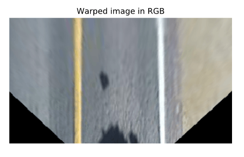
To HSL:
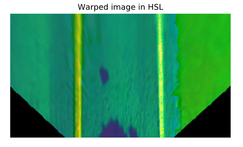
It certainly doesn't seem any easier to distinguish the lane lines from the HSL image than the RGB image, it actually seems a bit harder, until we split the image into three separate channels:
# Split the image into three variables by the channels
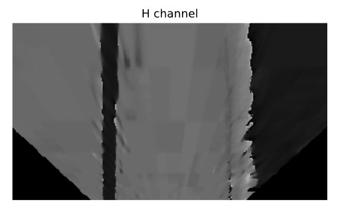
hChannel, lChannel, sChannel = cv2.split(hslImage)
showTitledImage("H channel", hChannel)
showTitledImage("L channel", lChannel)
showTitledImage("S channel", sChannel)
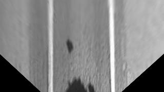
The hue channel doesn't look very helpful:
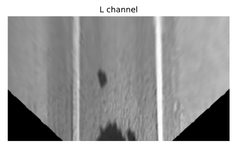
Neither does the lightness channel:
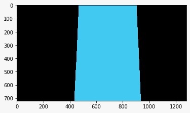
But the saturation channel certainly does:
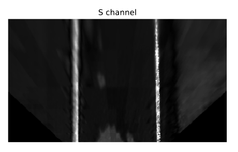
The reason for this is that the lane lanes are always saturated with color, be it white, yellow or any other color, which is what makes them stand out in the saturation channel, compared to the asphalt or the sand in the background.
We could've tried to find our lane lines by searching for pixels of a specific color, but that method would be far more susceptible to errors when the lane color changes due to light or weather conditions, or if we come across a lane that's just a bit differently colored than what we've expected, e.g. during construction.
This method is more robust since it doesn't care what color the lane line is, it just cares that it's really saturated with color.
There's one more thing we could do to make the lane lines pop out, as opposed to the lightly activated pixels on the asphalt, the sand on the right and the RC shadow in the middle of the lane. We could threshold the values of the saturation channel image, which basically means we'd only keep the pixels that are above a certain level of saturation, keeping only the most saturated pixels of the image.
That's pretty easy to do using OpenCV, and you can (and should) experiment with the threshold values by using a lot of different pictures of the road taken in different lighting conditions and of different lane line colors.
This is what the code looks like:
# Threshold the S channel image to select only the lines
lowerThreshold = 65
higherThreshold = 255

# Threshold the image, keeping only the pixels/values that are between lower and higher threshold
returnValue, binaryThresholdedImage = cv2.threshold(sChannel,lowerThreshold,higherThreshold,cv2.THRESH_BINARY)

# Since this is a binary image, we'll convert it to a 3-channel image so OpenCV can use it
# Doesn't really matter if we use RGB/BGR/anything else
thresholdedImage = cv2.cvtColor(binaryThresholdedImage, cv2.COLOR_GRAY2RGB)
showTitledImage("Thresholded S channel", thresholdedImage)
Note that the thresholded image will be a binary image, which means that any pixel that was above (or below) our threshold value (i.e. the pixels that we kept) will have a value of 255, which is the maximum value for the color channel (we're using the 0-255 range).
So the output image will look like this:
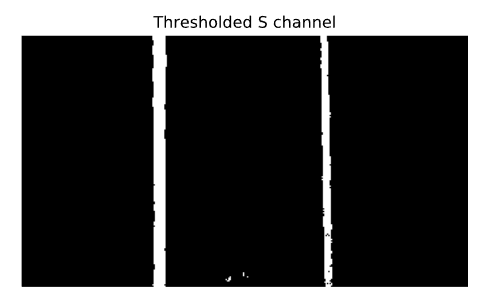
The white pixels are the ones that had a value larger than 65 in the original saturation channel image, and their value is 255 on the above image. The rest of the pixels which didn't cross the lower threshold were discarded and their value was set to 0, which is black in the image above.
We can now feed this image into our network and it'll be much easier for it to find the lane lines.
The entire process visualized
This is what the entire process would look like, in a video:
We also could've used a number of different approaches as opposed to our use of the S channel. We also could've combined multiple of them. A lot of people do. Let's go through some of them and I'll explain why I didn't use them.
Fitting lanes using a polynomial approximation
One thing I've seen a lot of people do, most of them during their Udacity Self-Driving Car Nanodegree program, is using a sliding window to find the lanes in an image processed in a way similar to ours, and fitting a polynomial to it.
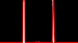
First, they would take the processed binary image and compute a histogram of the lower half of the image, to try and determine where the lane lines begin. This is what such a histogram would look like for our (entire, not just the bottom half) processed image:
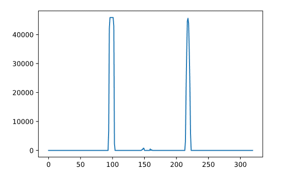
You can get the histogram by simply adding up the pixel values on the y axis, for each X-axis value. Here's the code:
# Sum the pixels on the x axis
# This will sum all pixel values for a given x axis (column)
histogram = np.sum(binaryThresholdedImage, axis=0)
plt.plot(histogram)
This is what it looks like overlaid on our processed image:
The method then splits the histogram into two parts, using the two X-axis that have the largest peak in the histogram as the starting positions for the two lane lines, and implements a sliding window search, going from the bottom up, that identifies the positions of all non-zero pixels on the image, and saves them into arrays.
After obtaining the four arrays, two for the left line (x and y) and two for the right one, it uses the numpy polyfit method to fit a polynomial to the line, and thus gets two polynomials that each define the lane.
Once the lanes are found in the first frame, the sliding windows don't go through the entire process again for the next frame. They use the previous frame as a starting position and use a margin at the top of the lane line to detect just the change from the first to the second frame, since it can't change that drastically from one frame to another.
The fitted polynomials can then be easily visualized, and since I've actually implemented this, this is what the result would look like in our simulator:
That looks pretty cool and works relatively well, so why not use it?
Well, I've tried to use it by passing on the fitted polynomials to the network, by passing the warped image with the detected lane overlaid on it:
and by passing the original image with the detected lane overlaid on it
The two main issues with the method are:
- It's computationally expensive to do all of the processing and fitting for every single frame
- It can go haywire if your car moves the slightest out of the predefined ROI, and even if you quickly correct it, since it uses the previous frames as a start for the next one, to be more computationally efficient, it would take some time for it to correct itself. I've also tried not using the previous frame and doing all of the work for every single frame, and it takes a lot of computational power to do so.
Also, I wouldn't like my model to rely so much on feature engineering and extraction, I'd like it to be more robust, even if it means it will be harder to train or take longer to train. By simply passing our processed image to a small convolutional network, it should be able to get all the information it needs from it, and it should be way less computationally expensive in the long run, even if we've added a couple of additional convolutional layers to our model. Even if we passed the fitted polynomials to the network, we'd still have to train the network to learn how to interpret them, and taking into consideration the short tests I did, I believe it would be less robust and even more computationally expensive to do so.
Using additional preprocessing methods
Apart from transforming the perspective of our image and getting the thresholded S channel image, we could've also used a number of different techniques to make the lane lines more visible. One example would be using the Sobel operator, which allows us to take the derivative of an image in the x or the y direction.
I've tried a number of them, including Sobel, which I'll show below, and I've found that they wouldn't really help much, at least on my test data.
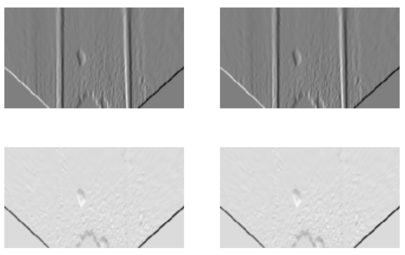
Here's an example of Sobel on both axes using these two input pictures:
Here's the images after applying the Sobel operator over both axes:
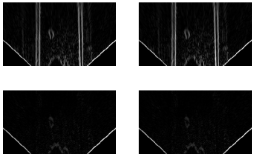
Here are the above images after np.absolute:
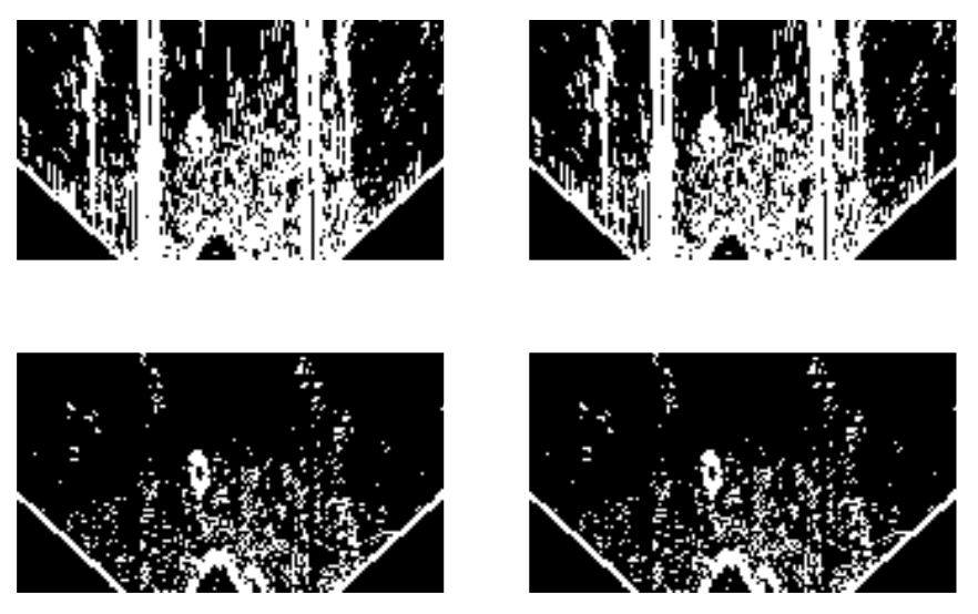
And here are the above images after applying a binary threshold on them, with the lower threshold being 200 and the upper 255:
Here's the code if you want to try it out for yourself:
def showSobelImages(images):
    f, axarr = plt.subplots(2,2)
    axarr[0,0].imshow(images[0], cmap='gray')
    axarr[0,0].axis('off')
    axarr[0,1].imshow(images[1], cmap='gray')
    axarr[0,1].axis('off')
    axarr[1,0].imshow(images[2], cmap='gray')
    axarr[1,0].axis('off')
    axarr[1,1].imshow(images[3], cmap='gray')
    axarr[1,1].axis('off')


grayWarpedImage = cv2.cvtColor(warpedImage, cv2.COLOR_BGR2GRAY)
plt.imsave('graywarped.jpg', grayWarpedImage, cmap='gray')
plt.imsave('schannel.jpg', sChannel, cmap='gray')
# Taking the derivative on the X-axis
xAxisSobelWarped = cv2.Sobel(grayWarpedImage, cv2.CV_64F, 1, 0, ksize=5)
xAxisSobelSChannel = cv2.Sobel(grayWarpedImage, cv2.CV_64F, 1, 0, ksize=5)

# Taking the derivative on the Y-axis
yAxisSobelWarped = cv2.Sobel(grayWarpedImage, cv2.CV_64F, 0, 1, ksize=5)
yAxisSobelSChannel = cv2.Sobel(grayWarpedImage, cv2.CV_64F, 0, 1, ksize=5)

images = [xAxisSobelWarped, xAxisSobelSChannel, yAxisSobelWarped, yAxisSobelSChannel]
showSobelImages(images)

# Absolute values
showSobelImages([np.absolute(x) for x in images])

lowerThreshold = 200
higherThreshold = 255
thresholdedImages = []
for image in images:
    returnValue, image = cv2.threshold(np.absolute(image), lowerThreshold,higherThreshold, cv2.THRESH_BINARY)
    thresholdedImages += [image]
showSobelImages(thresholdedImages)